Roland Young

During my DPhil I worked with the thermally-driven rotating annulus (right), a laboratory analogue for a generic planetary atmosphere. We can use the annulus to study methods for forecasting or data assimilation in current use or in development using a real fluid with a non-idealised model under laboratory conditions. The laboratory is a bridge between analytical systems, where new methods are first tested, and large atmospheric models, where they are eventually applied.

Baroclinic instability is an important mechanism for the development of large-scale waves and eddies in the atmospheres of the Earth (left) and other planets such as Mars. These waves and eddies are associated with the large-scale transport of heat and momentum; their chaotic evolution in the Earth's atmosphere determines the fundamental limit on how far ahead it is possible to forecast weather and (to a lesser degree) the climate. On Mars, however, baroclinic weather systems are significantly more coherent, and at times its atmosphere appears to be more predictable than the Earth's.

This research had three main aims:

Of the two kinds of predictability identified by Lorenz (1975), predictability of the "second kind" - i.e. the "climate" problem: determining the type of flow observed for a particular experimental setup - had already been well characterised for the rotating annulus over several decades. Predictability of the "first kind", however - i.e. the "weather" problem: predicting the evolution of a particular flow over time from a given initial state - had not been well explored until this work.

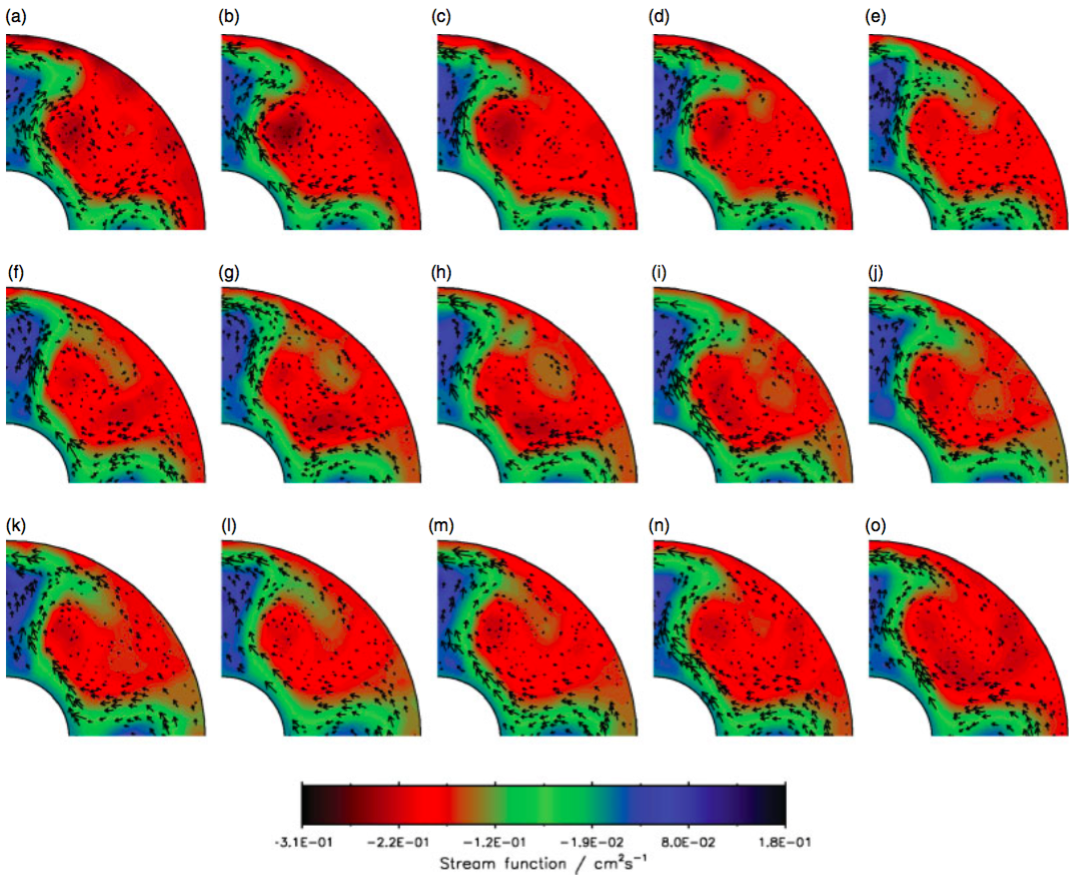
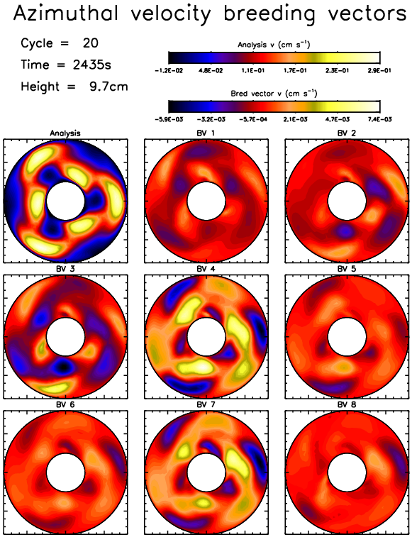
The intrinsic predictability of the most important quasi-periodic and chaotic flow regimes observed in the laboratory was investigated using numerical simulations with MORALS, the Met Office/Oxford Rotating Annulus Laboratory Simulation (Young & Read, 2008a). To determine the most unstable flow patterns we used the breeding vector method, which is a well-established technique for evaluating the intrinsic predictability of the state of the Earth's atmosphere and has been used by several operational weather forecasting centres worldwide in their everyday weather forecasts. The mechanisms causing predictability to break down were then studied using ensemble prediction techniques (Young & Read, 2008b). We used the analysis correction method to assimilate data into the model (Young & Read, 2013) in order to create initial states for our prediction experiments (Young, 2010, Young & Read, 2016).

The rotating annulus is a classic laboratory experiment that has been used since the 1950s to study fluid flows whose dynamics are similar to airflow in the midlatitudes of planetary atmospheres.

The experiment rotates about a vertical axis and is heated at the vertical boundaries of the fluid, generating a horizontal temperature gradient across the fluid. This is similar to the atmosphere, which is heated by the Sun more at low latitudes than at high latitudes (below), and also rotates about an axis. By changing these two parameters in the experiment a wide range of behaviour can be seen, from simple waves (right) to turbulence and chaotic flow. In this sense it is similar to the Earth's atmosphere.

Using the annulus avoids much of the complicated behaviour seen in the atmosphere, such as the difference between land and sea, the chemistry of different molecules in the air, and the biosphere. These effects are secondary to rotation, gravity, and heating, although some later experiments have included them. This simplicity makes it easier to study the physics behind weather and climate. The laboratory context also allows interpretation of the system behaviour without the difficulties associated with imperfect and incomplete observations of atmospheric circulation, and avoids some of the complexities resulting from a wide range of interacting scales and sub-systems.

In Young & Read (2013) we used the analysis correction method to assimilate laboratory measurements of fluid velocities into MORALS. The dataset containing these measurements is available via ORA-Data. We analyzed the 2S (steady flow, azimuthal wavenumber 2) and 3AV (amplitude vacillating) regular flow regimes, and the 3SV (structural vacillation) weakly chaotic flow regime at higher rotation rates.

The assimilated horizontal velocities were combined with the model to produce model states that were both consistent with our physical understanding (as represented by the numerical model) and consistent with the observations. As well as showing that data assimilation worked in this context, we examined a number of specific scenarios:

By using unobserved variables that are only available via the assimilation (such as temperature and the vertical structure of the velocity field), we found that the mean azimuthal flow is weakened by the action of eddies, which partly explained why vortices were shed at the very highest rotation rates but not at lower rotation.

In Young & Read (2016) we used our ensemble prediction system with breeding vectors and data assimlation to forecast the rotating annulus in steady 2S, amplitude vacillating 3AV, and structurally vacillating 3SV flow regimes, verifying the forecasts against laboratory data.

The steady wave flow regime was predictable until the end of the available data. Forecasts in the amplitude and structural vacillation flow regimes lost quality and skill by a combination of wave drift and wavenumber transition. Amplitude vacillation was predictable up to several hundred seconds ahead, and structural vacillation was predictable for a few hundred seconds. The wavenumber transitions were partly explained by hysteresis in the rotating annulus experiment and model.

I gave a talk to the general public about the lab experiments called Spin Doctors: Creating a planet's atmosphere in the lab at the 2014 Stargazing Oxford event. The video is online at University of Oxford podcasts and also at iTunes U.